On R-Squared and Economic Prediction

Recently I’ve heard a number of otherwise intelligent people assess an economic hypothesis based on the R² of an estimated regression. I’d like to point out why that can often be very misleading.

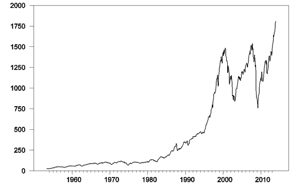
Value of S&P 500 index, 1953:M4 – 2013:M12. Data source: Robert Shiller.

The above graph plots the S&P500 stock price index since 1953. Here’s what you’d find if you calculated a regression of this month’s stock price (p_t) on last month’s stock price (p_t-1). Standard errors of the regression coefficients are in parentheses.

The adjusted R-squared for this relation is 0.997. One minus the R-squared is basically a summary of how large on average the squared residual of the regression is relative to the squared difference of the stock price from its historical mean. The latter is huge. For example, in December the S&P500 reached 1808, compared to its sample mean of 459. The square of that difference is (1808 – 459)² = 182,000, which completely dwarfs the average squared regression residual (25² = 625). So if you’re a fan of getting a big R-squared, this regression is for you.

On the other hand, another way you could summarize the same relation is by using the change in the stock price (Δp_t = p_t – p_t-1) as the left-hand variable in the regression:

This is in fact the identical model of stock prices as the first regression. The standard errors of the regression coefficients are identical for the two regressions, and the standard error of the estimate (a measure of the standard deviation of the regression residual e_t) is identical for the two regressions because indeed the residuals are identical for every observation. Yet if we summarize the model using the second regression, the R-squared is now comparing those squared residuals not with squared deviations of p_t from its sample mean, but instead with squared deviations of Δp_t from its sample mean. The latter is much, much smaller, so the R-squared goes from almost one to almost zero.

Whatever you do, don’t say that the first model is good given its high R-squared and the second model is bad given its low R-squared, because equations (1) and (2) represent the identical model.

This is not simply a feature of the trend in stock prices over time. Here for example is a plot of the interest rate on 10-year Treasury bonds, whose values today are not that far from where they were in the 1950s:

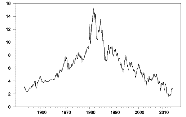
Interest rate on 10-year Treasuries, 1953:M4 – 2013:M12. Data source: Fred.

If you regress the interest rate on its values from the previous three months, you will get an R-squared of 0.992.

Or if you wanted to, you could describe exactly the same model by using the change in interest rates as the left-hand variable and report an R-squared of only 0.136:

Note by the way that regression (2) above reproduces a common finding, which is, if you regress the change in stock prices on most variables you could have known at time t – 1, you usually get an R-squared near zero and coefficients that are statistically indistinguishable from zero. Is the failure to get a big R-squared when you do the regression that way evidence that economists don’t understand stock prices? Actually, there’s a well-known theory of stock prices that claims that an R-squared near zero is exactly what you should find. Specifically, the claim is that everything anybody could have known last month should already have been reflected in the value of p_{t -1}. If you knew last month, when p_t-1 was 1800, that this month it was headed to 1900, you should have bought last month. But if enough savvy investors tried to do that, their buy orders would have driven p_t-1 up closer to 1900. The stock price should respond the instant somebody gets the news, not wait around a month before changing.

That’s not a bad empirical description of stock prices– nobody can really predict them. If you want a little fancier model, modern finance theory is characterized by the more general view that the product of today’s stock return with some other characteristics of today’s economy (referred to as the “pricing kernel”) should have been impossible to predict based on anything you could have known last month. In this formulation, the theory is confirmed– our understanding of what’s going on is exactly correct– only if when regressing that product on anything known at t – 1 we always obtain an R-squared near zero.

This is actually a feature of a broad class of dynamic economic models, which posit that some economic agent– whether it be individual investors, firms, consumers, or the Fed– is trying to make the best decisions they can in an uncertain world. Such dynamic optimization problems always have the implication that some feature of the data– namely, the deviation between what actually happens and what the decision-maker intended– should be impossible to predict if the decision-maker is behaving rationally. For example, if everybody knew that a recession is coming 6 months down the road, the Fed should be more expansionary today in hopes of averting the recession. The implication is that when recessions do occur, they should catch the Fed and everyone else by surprise.

It’s very helpful to look critically at which magnitudes we can predict and which we can’t, and at whether that predictability or lack of predictability is consistent with our economic understanding of what is going on. But if what you think you learned in your statistics class was that you should always judge how good a model is by looking at the R-squared of a regression, then I hope that today you learned something new.

• Create Content With AI
• Become A Funded Futures Trader