Is QE Lowering the Rate of Inflation?

The answer may be “yes,” according to a new paper by Steve Williamson. In examining the effects of a QE experiment in his model economy, he reports the following (p. 16):

Some of the effects here are unconventional. While the decline in nominal bond yields looks like the “monetary easing” associated with an open market purchase, the reduction in real bond yields that comes with this is permanent, and the inflation rate declines permanently. Conventionally-studied channels for monetary easing typically work through temporary declines in real interest rates and increases in the inflation rate. What is going on here? The change in monetary policy that occurs here is a permanent increase in the size of the central bank’s holdings of short-maturity government debt – in real terms – which must be balanced by an increase in the real quantity of currency held by the public. To induce people to hold more currency, its return must rise, so the inflation rate must fall. In turn, this produces a negative Fisher effect on nominal bond yields, and real rates fall because of a decline in the quantity of eligible collateral outstanding, i.e. short maturity debt has been transferred from the private sector to the central bank.

Williamson describes these findings on his blog here: Liquidity Premia and the Monetary Policy Trap.

Well, it must have been a slow news day on the economics front. The normally mild-mannered Nick Rowe set off a tempest in a teapot when he wondered out loud what “went the hell went wrong with the best and brightest in the profession?”  Nick’s little tirade was then picked up by the charming duo of Brad DeLong and Paul Krugman.

So what happened? It all started out by Williamson discussing two “fearsome equations” that emerge as theoretical restrictions in a wide class of macroeconomic models. Some people call these restrictions “Fisher equations.” I like to think of them as no-arbitrage-conditions.

Let’s make some assumptions. There is no uncertainty. We are (the model economy is) in a state-state, so that output grows at the gross rate G. The level of output may be above or below its “natural” level (the level that would prevail if all frictions were absent). Let B denote the discount factor. Absent all frictions, the “natural” rate of interest is given by (G/B).

Let P denote the gross rate of inflation. There are two nominal assets, a bond that yields a gross nominal return R >= 1, and money, which yields a gross nominal return equal to 1. Money is assumed to be more liquid than bonds (bonds cannot be used in a subset of transactions).

The “Fisher equations” that emerge from the model can be written as follows:

where K and L denote “liquidity premia.” In most models, K=1. In this case, the two equations above imply R = L. That is, the liquidity premium on money is equal to the nominal interest rate.

In the “newmonetarist” models that Steve studies, assets apart from money may serve in some manner as exchange media. If financial markets do not work perfectly well (say, because of limited commitment and asymmetric information frictions), then the supply of exchange media may be “scarce.” In the present context, this implies K>1, and equations [1] and [2] imply: R*K = L.

The traditional Friedman rule policy implies R = 1, K = L =1, so that P = (B/G). But Steve is assuming the government does not have enough instruments to implement the Friedman rule. In fact, he makes a distinction between the monetary and fiscal authorities. And, as he stresses in his paper (not his blog post), a lot hinges on exactly how one models this relationship.

One scenario that emerges in Steve’s model is R =1 and K = L > 1. In this case, the economy is at the ZLB, but government liabilities (cash and bonds — they are perfect substitutes in this case) exhibit a liquidity premium. On open market operation of cash for bonds in this case has absolutely no effect — this is the classic liquidity trap — something that Krugman stressed long ago. From [1] and [2], the equilibrium inflation rate is given by P = (B/G). The equilibrium real rate of interest on government liabilities is 1/P = G/(B*L), which is less than the “natural” real rate of interest (G/B). This is the sense in which the real rate of interest is “too low.” (Of course, if you have a different theory of the way the world works, you may be thinking that the real rate of interest is “too high”–but I’m not here to talk about that theory.)

Suppose that the bond we are talking about above is a short-maturity instrument. Imagine that the fiscal authority also issues a long-maturity instrument. Moreover, assume that this long-bond is less liquid than the short-bond (the short-bond is, in present circumstances, viewed as a perfect substitute for cash). Steve then asks what the model implies when the open market operation consists of a swap of cash for the long-bond. In this case, not surprisingly, QE matters. But how does it matter?

The effect of this policy in Williamson’s model is to lower the nominal interest rate at the long end of the term structure. Because the Fed is sucking out relatively less liquid assets and replacing them with relatively liquid assets, liquidity premia decline (as one would expect). So, if we take a look at equation [2], we see that the model implies that inflation must decline: P = (B*L)/G. What is the economic intuitions for this? Evidently, one of the effects of QE (in the model) is to increase the real stock of currency held by the private sector, and agents require an increase in currency’s rate of return (a fall in the inflation rate) to induce them to hold more currency. (Remember that the results are all contingent on the way monetary and fiscal policy are modeled.)

So this is kind of interesting for a couple of reasons. First, the model offers an explanation for why we do not observe deflation, given that we are at the ZLB (a bit of a puzzle, for conventional theory.) Second, it offers an explanation for how QE may be putting downward pressure on inflation. How quantitatively important these effects are relative to others remains an open question.

Krugman and DeLong seem to want to argue that Williamson’s results are “incorrect” because the model equilibrium he is focusing on is “unstable.” I’m pretty sure I know where they’re coming from, but I’m not sure that the criticism applies here.

First, to demonstrate the “stability properties” on an equilibrium, one actually has to go and work out the math. I think it’s fair to say that nobody has done that.

Second, what Krugman writes in his “Little Arrows” post is correct, but it is correct only in the context of a particular theory. As I’ve mentioned before, Peter Howitt demonstrates here how pegging the nominal interest rate is unstable under a wide class of algorithms that govern the manner in which inflation expectations are formed (essentially, adaptive expectations). This led Howitt to argue that stability required a policy to raise interest rates more than one-for-one with inflation expectations. Hence, Howitt came up with the “Taylor principle” before Taylor did.

It is interesting to note, however, that the “stability properties” induced by the Taylor principle in standard New Keynesian models (which embed rational expectations) is something very different. At the opposite extreme, one might take the view that inflation expectations are formed in a manner described here, by Stephanie Schmitt-Grohe and Martin Uribe. Let me reproduce the diagram I used in that blog post here:

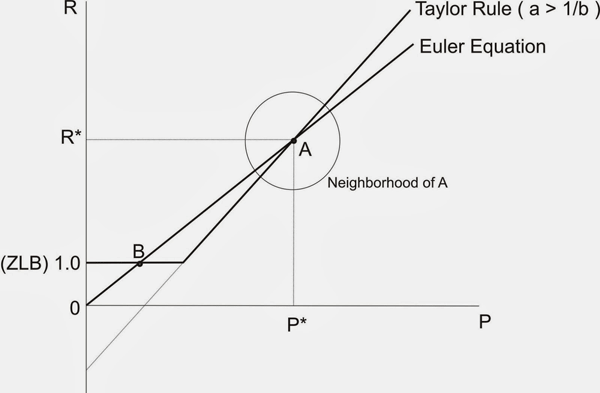
As you can see, it is identical to Krugman’s “Little Arrows” diagram. The one big difference here is that–under this particular theory of expectations formation–rational expectations–A is unstable and B is stable. So the “little arrows” run in the opposite direction here.

The little circle in the picture above demonstrates how the New Keynesians use the “Taylor principle.” Essentially, they restrict attention to trajectories around the steady state point A that never leave that circle. If the Fed follows the Taylor principle, then there is only one point that satisfies this property, and it is point A. Viola-we say that point A is “locally stable” (Yes, I know it sounds weird, but I’m just reporting the facts.) In their Perils of Taylor Rules, Benhabib, Schmitt-Grohe, and Uribe argue that only point B (the liquidity trap) is globally stable. (The fact that Japan has spent decades around a point like B suggests that it may in fact be stable.)

The other thing I’d like to add is that Williamson’s results continue to hold even away from the ZLB. So, Krugman’s post in particular, which focuses on the properties of Taylor rules (absent in Williamson’s model) seems a little off target.

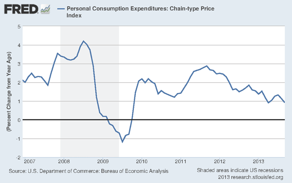
So my interpretation of the criticisms I am hearing of Williamson’s paper is that his critics are claiming that he is wrong because his results are inconsistent with the type of models these people are used to working with. It seems to me that the critics should have instead attacked his results and interpretations with empirical facts (or am I too old-fashioned in this regard?). After all, Williamson at least motivated his post with some data (the diagram at the top of this post). And he makes what is potentially a testable prediction (notice the if-then structure of the statement):

In general, if we think that inflation is being driven by the liquidity premium on government debt at the zero lower bound, then if the Fed keeps the interest rate on reserves where it is for an extended period of time, we should expect less inflation rather than more.

I have a little more difficulty in understanding Nick Rowe’s objection. Certainly, a part of it seems to be what I just described above. Partly, I think that Nick is disagreeing not with Williamson’s model, but with the way Williamson seems to run off at the end of his post with his “the Fed is in a trap” ideas.

And so, this now leads me to my own criticism of Williamson’s post.

I wish he had spent a little more time elaborating on this statement he makes:

But the power of monetary policy to mitigate the inefficiency is limited. Basically, it’s a fiscal problem. The U.S. government could issue more debt, by temporarily running a higher deficit. But that’s not happening, so what can the central bank do about it?

It’s a fiscal problem (well, the fundamental problem is limited commitment and asymmetric information in these models). The Treasury could alleviate the “asset shortage” by expanding the supply of Treasury debt! I discussed this idea here some time ago: Not Enough Debt? So isn’t this nice? Different models, but similar policy conclusions. Implicitly, Williamson is taking the view that political constraints are preventing this from happening, so let’s move on to study Fed policy.

The tone of his post near the end strikes me as odd. He seems rather critical of the way Fed economists generally think about the way monetary policy works. Fair enough. On the other hand, if we read his paper we find the following statement:

QE is a good thing, as purchases of long-maturity government debt by the central bank will always increase the value of the stock of collateralizable wealth.

That is, QE is a good thing in his model economy. In fact, I think his model suggests that the Fed should buy up all outstanding treasury debt (but that even that would not be enough because the problem is the limited supply of the stuff).

So what’s his problem? Well, it seems that conventional Fed thinking is that QE is inflationary and, well, as Williamson’s paper shows, it may have the opposite effect. O.K., well, so what?

Then Williamson remarks that if the Fed really wants inflation, it should raise its policy rate (IOER). This, of course, is the statement that drew all sorts of criticism when Narayana Kocherlakota suggested something similar a few years back (thanks to Nick Rowe for once again starting that one). Williamson believes that raising the policy rate would be disruptive in the short-run, but that this is the way to achieve higher inflation in the long-run. I am not sure, however, whether his model suggests that higher inflation is a good thing (I don’t think so.) These are all positive (not normative) statements.

So, the Fed is “stuck.” That is, the Fed seems compelled to continue QE and keep the IOER at 0.25%. Williamson’s model seems to suggest this is a good thing. But his model also suggests that the policy is ultimately deflationary (perceived to be a bad thing). The only way to prevent this trajectory is to raise the IOER (another way would be to expand the supply of treasury debt). But doing so will cause a recession because of monetary non-neutralities.

Not sure what any of this has to do with eating more crow though. What would the Fed be doing differently if they took this view? Not much, as far as I can see.