U.S. Imports, Exports: The Collapse Continues

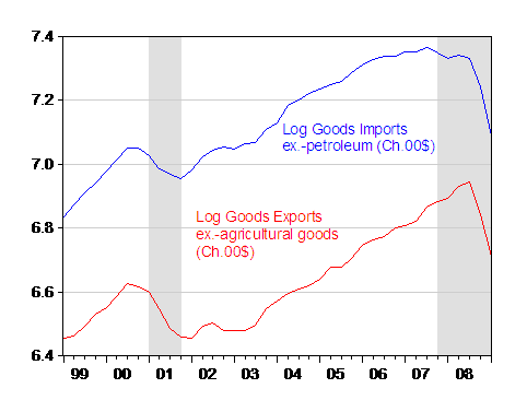
Here’s an update of US imports and export behavior. The trade collapse remarked upon a couple of months ago is still in play.

Figure 1: Log goods import ex.-oil from NIPA (blue), and log goods exports ex.-agricultural goods (red), all in Ch.2000$, SAAR. NBER recession dates shaded gray. Source: BEA, GDP 2009Q1 preliminary release of 28 May 2009, NBER, and author’s calculations.

The annualized drop in non-oil goods imports was 60.5% in 2009Q1 (log terms), while that of non-agricultural goods exports was 51.5% (both in log terms).

The misprediction by the standard (i.e., old fashioned) macroeconometric models (see [1]) documented in an earlier post persists. The model is given by:

Imp = α 0 + α 1 y + α 2 r

Where Imp is real imports, y is real income, and r is the real value of the dollar.

I estimate an error correction version of this model over the 1973q1-2009q1 period, wherein there is a long run relation between the levels of imports, income and the real dollar.

Δ imp t = β 0 + φ imp t-1 + β 1 y t-1 + β 2 r t-1 + γ 1 Δ imp t-1 + γ 2 Δ y t-1 + γ 3 Δ r t-1 + u t

In this specification, the long run elasticities are given by the ratio β i/ φ . When this model is estimated over the 1974q1-2008q4 period, one obtains sensible estimates (in that higher income or a stronger dollar induces greater imports in the long run).

The specification fits fairly well, with an adjusted R-squared of 0.34, and a Breusch-Godfrey Serial Correlation LM Test (2 lags) failing to reject the null at conventional levels. The long term coefficients are statistically significant, while the reversion coefficient (φ) is also significant and negative.

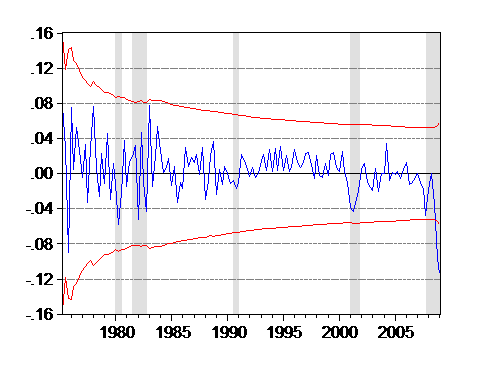
One way of evaluating whether the 2008q4-09q1 observations are anomalous, in a statistically significant sense, is to examine the recursive residuals. A recursive residual is the time t prediction error based upon the regression estimated up to time period t-1, but using time t values of the X variables. Figure 2 depicts the 95% standard error band; an observation outside that band suggestive structural instability in the regression equation.

Figure 2: Recursive residuals from standard model of imports error correction specification, 1974q1-2009q1. +/- two standard error band (red dashes).

What about exports? I estimate an analogous expression for non-agricultural goods exports.

Δ exp t = θ 0 + ρ exp t-1 + θ 1 y* t-1 + θ 2 r t-1 + σ 1 Δ exp t-1 + σ 2 Δ y* t-1 + σ 3 Δ r t-1 + v t

Note that the rest-of-world GDP variable (y*) is the export weighted real GDP calculated by the Federal Reserve Board, for 1970q2-07q4; the 2008q1-09q1 data I estimated using a regression of first differenced GDP on a current and four lags of first differenced industrial country industrial production.

(Data sources: BEA 2009q1 preliminary release for imports, exports, GDP; Federal Reserve Board for broad index of real dollar value; personal communication/Fed for rest-of-world export weighted GDP; and IMF International Financial Statistics for industrial country industrial production (nsa).)

This specification also fits fairly well, with an adjusted R-squared of 0.34, and the serial correlation test again failing to reject. The long run coefficients are significant, as is the reversion coefficient (ρ).

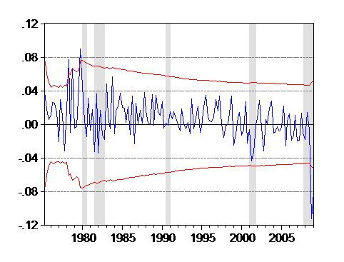
Recursive residuals indicate a similar misprediction for 2008q4-09q1.

Figure 3: Recursive residuals from standard model of exports error correction specification, 1974q1-2009q1. +/- two standard error band (red dashes).

For speculation regarding the causes of this downturn, see [1]. Detailed regression results downlodable here [pdf].

Update on US Exports and Imports: The Collapse Continues

• Become A Funded Futures Trader