The world’s current economic problems started when housing bubbles burst in several advanced economies. Economic recovery without housing market recovery is unlikely to be sustained. This column presents new research on the probability of housing slumps ending. There is at least a one-in-eight chance of housing slumps in the three big economies (US, Japan and Germany) ending imminently, but there is nothing approaching the same probability elsewhere. If things turn out as projected here, we may be about to have a test of the locomotive theory – whether the big economies can pull along their smaller brethren – both for housing markets and generally.
As concern over the sustainability of public debts has risen to the top of the list of macroeconomic concerns, it has become too easy to forget that this crisis started with a housing slump (Cecchetti 2007). How it ends will also depend, in part, on housing markets.
Construction is a particularly volatile component of economic activity. Changes in house prices can powerfully impact consumer confidence. House-price developments have obvious implications for bank balance sheets and the condition of financial institutions. All these are reasons for worrying that economic recovery without housing-market recovery is unlikely to be sustained.
How house prices now develop in different countries will, of course, depend on country-specific circumstances. But it is nonetheless possible to pick out some general patterns in how housing slumps end, and why.
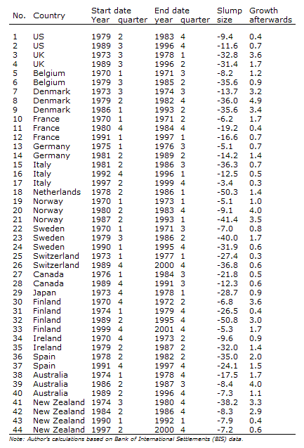
In recent research, we define the start of a slump as the point in time where the house price index adjusted for inflation is at a local maximum, and its end as the local minimum. To declare a slump definitively over, we also require inflation-adjusted prices to rise on average for four subsequent quarters. Our method identifies 44 slumps (shown in the appendix) with both start and end dates between 1970Q1 and 2009Q1 (Bénétrix, Eichengreen, and O’Rourke 2010).
Five variables go a long way toward explaining whether a slump is poised to end:
- The cumulative rise in house prices prior to the slump. This captures the idea that the duration of a house price bust should be related to the size of the preceding boom.
- The cumulative house price fall during the slump. If slumps involve the realignment of prices to sustainable levels, then the probability of their ending will depend on how much of that price adjustment has taken place.
- GDP growth in the current quarter, previous studies finding a tight relationship between housing prices and the business cycle.
- Mortgage interest rates in the current quarter as a measure of the cost of housing finance.
- Private credit growth during the current year as a way of capturing access to credit.
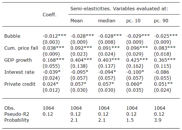
We estimated this model on quarterly data for 18 countries (Table 1).
Table 1: Baseline probit model

Note: Probit model estimated using a dummy variable taking value one in each slump end date and zero otherwise. Country fixed-effects included. *, ** and *** indicate statistical significance at 10%, 5% and 1% levels, respectively. Robust standard errors in parentheses. Semi-elasticities are the percentage change in the probability of bottoming out in response to a one unit change in the explanatory variable.
All five variables have their expected effects. The impact of previous house price booms on the probability of a slump ending in the current quarter is negative and significant. A 1 percentage point increase in the house price boom reduces the probability of bottoming out in the current quarter by 2.5 to 2.9%. Similarly, the cumulative house price fall has a positive effect on the probability of the slump ending. A 1 percentage point increase in the cumulative fall (relative to the level at the start of the slump) increases the probability of bottoming out by 8.3-9.6 percent.
Output growth has a negative effect on the duration of the slump. On average a 1 percentage point increase in output growth rates raises the probability of bottoming out in the current quarter by 36.5 to 42.5 percent.
Financial conditions also matter. A one percentage point increase in the real mortgage rate reduces the probability of a slump ending by 8.6-10%. Private credit growth as a measure of access to finance has the opposite effect: a 1 percentage point increase in the growth rate of private credit during the slump increases the probability of prices bottoming out by 5.1-6 %.
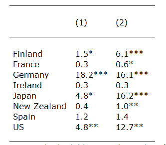
Table 2 uses the latest data for 2010Q1 on GDP growth and mortgage interest rates to estimate the likelihood that housing slumps in different countries will now come to an end. The countries where this is most likely are Germany, Japan and the U.S. Germany never saw much of a housing bubble and has now registered relatively strong GDP growth. Japan has seen a very large house-price decline, has low mortgage rates, and has recently shown signs of stronger growth. Similar conditions make for a 13 per cent probability that the U.S. housing slump will end in the current quarter. (July’s exceptionally bad National Association of Home Builders confidence survey for the U.S. reminds us than one in eight is less than one.)
The model also points to a statistically significant probability of housing slumps now ending in Finland, France and New Zealand, but the likelihood of this happening in the last two countries is so small as to be economically negligible.
At the other end of the spectrum are countries like Spain and Ireland which experienced big housing bubbles and now big economic slumps, with no great prospects for immediate economic recovery. Our estimates suggest that ongoing housing slumps will continue to add to their woes. The 3.6 per cent year-on-year fall in Spain in the recently-completed second quarter of the year is consistent with this prediction. So is the 4.2 per cent decline in asking prices for Irish residential properties in the same period.
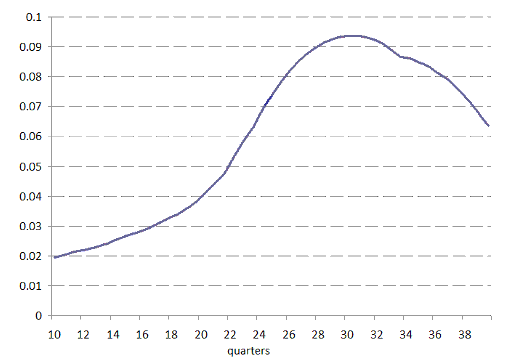
On the other hand, allowing prices to adjust downwards rapidly in these countries is the best way to ensure that they eventually stop falling, given the importance of our “cumulative price fall” variable. In some further results, we find that the probability of exiting a slump declines after it has been ongoing for 30 quarters (see Figure 1). If price adjustment is needed, it is important to let that price adjustment take place.
Figure 1: Hazard function

Note: Smoothed hazard function generated by a Cox proportional hazard model. Estimated using the above five explanatory variables. Vertical axis measures the hazard of a slump end.
Table 2: Predicted end probabilities for ongoing slumps

Note: Simulated probabilities using latest values of all variables by country. Column (1) uses data for 2009Q1, which is included to estimate the baseline model. Column (2) uses OECD latest estimates for GDP growth in 2010Q1 and IMF mortgage rates for 2010Q1 or 2009Q4 where available. *, ** and *** indicate statistical significance at 10%, 5% and 1% respectively.
Conclusions
The good news, then, is that there is at least a one-in-eight chance of housing slumps in the three big economies ending imminently, which in turn will be positive for economic growth. The bad news is that there is nothing approaching the same probability elsewhere. If things turn out as projected here, we may be about to have a test of the locomotive theory – whether the big economies can pull along their smaller brethren – both for housing markets and generally.
References
Agustín Bénétrix, Barry Eichengreen, and Kevin H. O’Rourke (2010), “How Housing Slumps End”, mimeo.
Appendix
House price slumps (inflation-adjusted prices)

![]()


Leave a Reply